Default Risk Modeling
Data Analysis and Modeling

Introduction
Home Credit is looking for a model to predict the possibility of loan repayment for their clients based on the information about applicants’ applications, credit card history, account balance and etc. The dataset contains of 7 relational tables.
In my analysis, I will stick to using the main application training and testing data which should be more manageable. This will let me establish a baseline that I can then improve upon. With these projects, it’s best to build up an understanding of the problem a little at a time rather than diving all the way in and getting completely lost. Next I will use other tables to tune my model.
Literature Review
Credit risk management in banks essentially focuses on determining likelihood of client’s default or credit deterioration and how costly it will turn out to be if it does occur (George, Sinha, Murali, 2007) . Decisions concerning credit granting are one of the most important in commercial banks’ policy. Well allocated credits may become one of the biggest sources of profits for banks. On the other hand, this kind of bank’s activity is connected with high risk as big amount of bad decisions may even cause bankruptcy. The key problem consists of distinguishing good (that surely repay) and bad (that likely default) credit applicants. The main investigations, in this area, are based on building credit risk evaluation models, allowing for automating or at least supporting credit granting decisions (Zakrzewska, 2007) . According to Lai, Yu, Wang, Zhou(2006) many different approaches including individual models, such as linear discriminant analysis, logit analysis, probit analysis, linear programming, integer programming, k-nearest neighbor, classification tree, survival analysis, artificial neural networks, genetic algorithm, support vector machine and some hybrid models are widely applied to credit risk analysis tasks . In this literature, I review some of these techniques and applications.
Gabriel and Rosenthal(1991) used probit analysis to evaluate the effects of borrower race and default risk in mortgage lending. The data include detailed information on the assets and liabilities of a nationally representative sample consisting of over 4,000 U.S. households. Using these data, a probit model of household mortgage loan choice was estimated by maximum likelihood. He found that non-whites are significantly less likely to obtain the conventional financing than whites. Therefore, race effects in the mortgage market. Lawrence and Smith(1991) , used logistic regression to evaluate risk of mobile home credit. The data includes more than 170,000 loans, which randomly are selected approximately 42,000 accounts that were active as of September 1, 1988. In that model, higher probabilities of loan default are associated with poor payment histories, smaller loans, higher current loan-to-value ratios, loans that have been in effect for shorter periods, lower initial income-to-payment ratios, older borrowers, higher statewide unemployment rates, areas having greater retail sales per household, and states having higher-priced mobile homes.
Boyes, Hoffman and Low(1989) suggested a model of credit assessment focuses on expected earnings. They demonstrated how maximum likelihood estimates of default probabilities can be obtained from a bivariate ‘censored probit’ framework using a ‘choice-based’ sample originally intended for discriminant analysis. His model demonstrates how expected earnings on revolving credit loans depend both on maintained balances and probability of default. The ‘choice-based’ estimator of Manski(1977) may then be combined with the notion of ‘partial observability’ to estimate default probabilities from non-random samples of consumer lending behavior originally intended for use in discriminant analysis. They also questioned the sample collection which samples used to estimate repayment probabilities are censored since only applicants that receive credit are observed to default or repay and there is no way to observe the subsequent behavior of the excluded group. Heckman has shown that censored samples can lead to biased estimates, if, in our example, the sample selection rule is correlated with the errors in the repayment probability equation. However, if lenders rely strictly on quantitative credit scores, sample selection is deterministically governed by applicant attributes and the sample selection rule does not lead to biased estimates while most lenders consider credit scoring as only one parameter of credit assessment procedure. Therefore, the standard Heckman procedure is not applicable. The data employed were obtained from a single large financial institution that monitored a non-random sample of its credit card applicants between 1977 and 1980 as well as the performance through 1984 of those granted credit. He found that variables which are significant (5% level) in both equations and carry opposite sign include age, number of dependents, post-baccalaureate education, home ownership, expenditures to income ratio, finance company reference, several credit bureau variables, number of months on the current job, between 13 and 15 years of education, home rental and department store credit card reference. He suggested instead of using credit scoring models, the complete model credit assessment would account for ‘time-to-default’ by applying split population survival time models of borrower behavior.
Srinivasan and Kim(1987) applied four statistical models: multiple discriminant analysis (MDA), logistic regression (logit), goal programming (GP) and recursive partitioning algorithm (RPA), and a judgmental model based on the Analytic Hierarchy Process (AHP). The data employed for the study has been provided by an anonymous Fortune 500 corporation. They found that (nonparametric) recursive partitioning methods provide greater information than simultaneous partitioning procedure and the judgmental model performs as well as statistical model.
Hillman(2014) used a binary logistic regression model to compare borrowers who defaulted against those who made standard “on‑time” repayments. The data is from Postsecondary Students (BPS) survey for 2003–2004 through 2008–2009. Participants in this survey (n ≈ 16,700) attended public, private nonprofit, and private for‑profit institutions in the United States and approximately 9,500 of the respondents had taken out federal student loans while enrolled in college. He found that students who attend for‑profit colleges are systematically (and to a greater magnitude) more likely to default than students attending other sectors of higher education. Also, students who come from upper‑income families or who are not first‑generation students face lower odds of defaulting. Alternatively, lower‑income students, minoritized students, and students who care for dependents face greater odds of defaulting when compared to their White and upper‑income peers who do not care for dependents.
Bellotti and Crook(2009) applied survival analysis to build the default model using credit card account dataset from a UK bank which includes a period of credit card accounts opened from 1997 to mid-2005 with the total number of 100,000 accounts with application variables such as income, age, housing and employment status along with a bureau score taken at the time of application. They showed that probability of default is affected by general conditions in the economy over time and these macroeconomic variables cannot readily be included in logistic regression models. However, survival analysis provides a framework for their inclusion as time-varying covariates. They believe that a credit application scoring model involves predicting the probability that an applicant will default over a given future time period in terms of characteristics of the applicant measured at the time of application. Moreover, although LR has become a standard method for estimating applicant scoring models (Thomas et al, 2002) , using survival analysis for credit scoring allows us to model not just if a borrower will default, but when. The advantages of this method are that
- survival models naturally match the loan default process and so incorporate situations when a case has not defaulted in the observation period
- it gives a clearer approach to assessing the likely profitability of an applicant
- survival estimates will provide a forecast as a function of time from a single equation
Survival analysis is used to study time to failure of some population. This is called the survival time. The results of the research demonstrate that survival analysis is competitive in comparison with LR as a credit scoring method for prediction.
Bastos (2010) used regression trees to evaluates the ability of a parametric fractional response regression and a nonparametric regression tree model to forecast bank loan credit losses. The dataset employed for this study is provided by the largest private bank in Portugal, Banco Comercial Português. The sample contains 374 loans granted to small and medium size enterprises that defaulted between June 1995 and December 2000. He evaluated the model with two different approaches: an out-of-sample estimation using the complete dataset with the help of a 10-fold cross-validation, and an out-of-time estimation in which the models are fit using defaults from one period and the accuracy is measured on defaults from the following year. When out-of-sample estimation is considered, the regression trees give better results for shorter recovery horizons of 12 and 24 months, while the fractional response regression gives better results for longer horizons.
Moulton, Haurin and Shi(2015) used bivariate probit model with sample selection to model default, given that households have a choice to select into a HECM. The data employed from a large nonprofit housing counseling organization (ClearPoint Credit Counseling Solutions) for the years 2006–2011 which includes demographic and socio-economic characteristics of the counseled, household credit score, outstanding balances and payment histories on revolving and installment debts, and public records information with total number of 27,894 applicants. The result shows that property tax is one the main reasons which causes the default.
Dataset
The dataset has 7 tables. In this project I will try to use other table than application table to refine my result. However, it depends on the time availability.
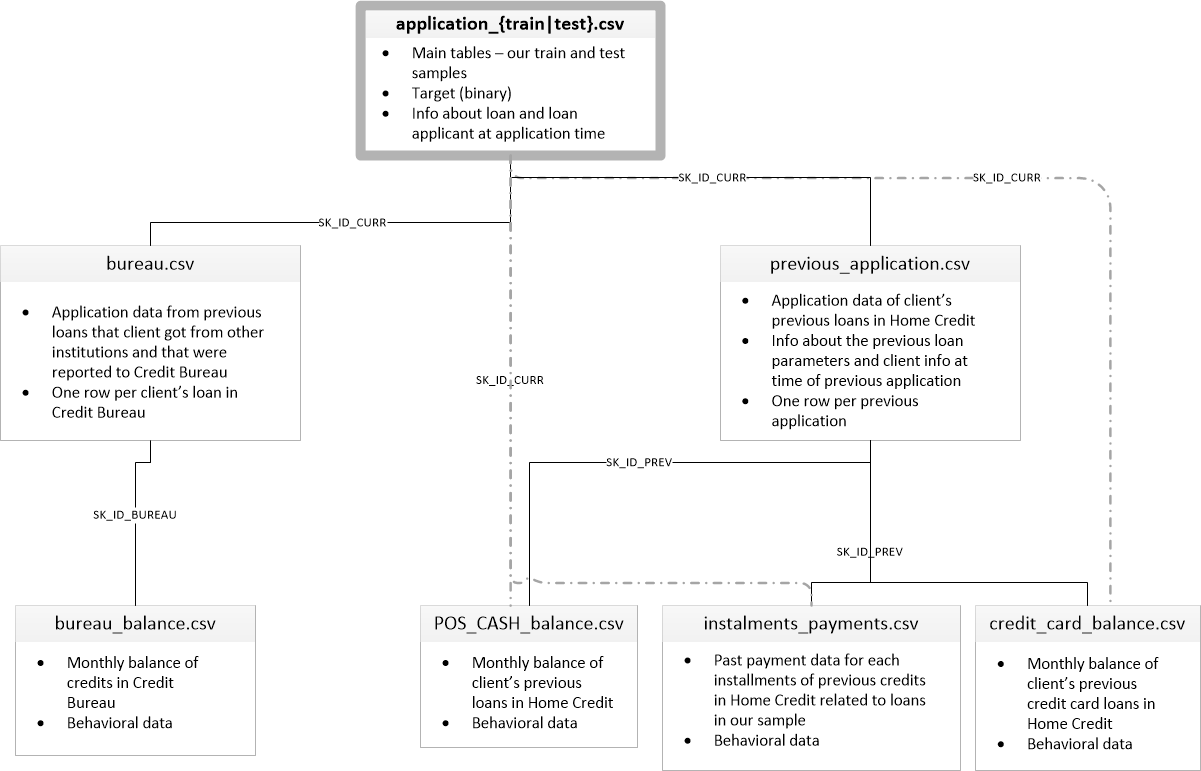
application_{train|test}.csv
- Size (train): 308k x 122
- Size (test): 48.7k x 121
- This is the main table, broken into two files for Train (with TARGET) and Test (without TARGET).
- Static data for all applications. One row represents one loan in our data sample.
bureau.csv
- Size: 1.72m x 17
- All client’s previous credits provided by other financial institutions that were reported to Credit Bureau (for clients who have a loan in our sample).
- For every loan in our sample, there are as many rows as number of credits the client had in Credit Bureau before the application date.
bureau_balance.csv
- Size: 27.3m x 3
- Monthly balances of previous credits in Credit Bureau.
- This table has one row for each month of history of every previous credit reported to Credit Bureau – i.e the table has (#loans in sample # of relative previous credits # of months where we have some history observable for the previous credits) rows.
POS_CASH_balance.csv
- Size: 10.0m x 8
- Monthly balance snapshots of previous POS (point of sales) and cash loans that the applicant had with Home Credit.
- This table has one row for each month of history of every previous credit in Home Credit (consumer credit and cash loans) related to loans in our sample – i.e. the table has (#loans in sample # of relative previous credits # of months in which we have some history observable for the previous credits) rows.
credit_card_balance.csv
- Size: 3.84m x 23
- Monthly balance snapshots of previous credit cards that the applicant has with Home Credit.
- This table has one row for each month of history of every previous credit in Home Credit (consumer credit and cash loans) related to loans in our sample – i.e. the table has (#loans in sample # of relative previous credit cards # of months where we have some history observable for the previous credit card) rows.
previous_application.csv
- Size: 1.67m x 37
- All previous applications for Home Credit loans of clients who have loans in our sample.
- There is one row for each previous application related to loans in our data sample.
installments_payments.csv
- Size: 13.6m x 8
- Repayment history for the previously disbursed credits in Home Credit related to the loans in our sample.
- There is a) one row for every payment that was made plus b) one row each for missed payment.
- One row is equivalent to one payment of one installment OR one installment corresponding to one payment of one previous Home Credit credit related to loans in our sample.
HomeCredit_columns_description.csv
- Size: 219 x 5
- This file contains descriptions for the columns in the various data files.
Results
Exploratory Data Analysis
By doing EDA some information has been extracted from the application data set as below:
We can infer that younger people may experience more default than elders.


Correlation Heatmap between top features and Target

All three EXT_SOURCE features have negative correlations with the target, indicating that as the value of the EXT_SOURCE increases, the client is more likely to repay the loan. We can also see that DAYS_BIRTH is positively correlated with EXT_SOURCE_1 indicating that maybe one of the factors in this score is the client age.

Modeling
Several model had been built to check the accuracy and the score given by Kaggle. The below is the result of each method:
1st Model: Logistic Regression
As building my baseline model, I used Logistic Regression from Scikit-Learn library. I used only the main table (Application) to build the model.
- Result: This scores 0.68035 when submitted which probably shows that the engineered features do not help in this model.
2nd Model: Random Forest
The second model was built on the same dataset to figure out the feature importance as show below.

As expected, the most important features are those dealing with EXT_SOURCE and DAYS_BIRTH. We see that there are only a handful of features with a significant importance to the model, which suggests we may be able to drop many of the features without a decrease in performance (and we may even see an increase in performance.)
- Result: This model score is 0.67508 when submitted. No progress in score!
3rd Model: Application Data set and Light Gradient Boosting
In this step I only create Light Gradient Boosting control model to compare the further step results with it. The score of 0.74533 reached when submitted the result.
- Result: The control slightly overfits because the training score is higher than the validation score.
| fold | train | valid |
|---|---|---|
| 0 | 0.809199 | 0.760273 |
| 1 | 0.812654 | 0.761398 |
| 2 | 0.809734 | 0.750451 |
| 3 | 0.811121 | 0.760245 |
| 4 | 0.802236 | 0.760972 |
| overall | 0.808989 | 0.758635 |

4th Model: Manual Feature Engineering and Light Gradient Boosting
The objective of feature engineering is to create new features to represent as much information from an entire dataset in one table. In this modeling I joint the bureau and bureau_balance table to the application table and calculated the correlations. This correlation Heatmap shows that some of the new created values from bureau data set has some correlation with target.

The data set dimension increased from 122 to 333 columns. To decrease the number of features the method below were used:
1- Missing Values: If a column has more than 90% of missing values, it should be removed.
- Result: No column has been removed.
2- Collinear Variables: If two variable has strong correlation one should be removed.
- Result: 134 of columns to remove. Also 53% of top 100 features created from the bureau data.
For modeling I used light gradient boosting to build our model. First I build a model with the 333 columns and then built it again after removing 134 columns. At the end I joint all tables application and build a giant one and build a model based on that.
5th Model: Automated Feature Engineering and Light Gradient Boosting
In these step I used featuretools library. Automated feature engineering aims to help the data scientist with the problem of feature creation by automatically building hundreds or thousands of new features from a dataset. The data dimensions increased to 2221 features. Many of the have collinearity with each other and those over 90% were removed.
As an example: MEAN(credit.AMT_PAYMENT_TOTAL_CURRENT)) and MAX(previous.MEAN(credit.AMT_PAYMENT_TOTAL_CURRENT) have 0.9998 correlation.
Result of the modeling
The score of 0.74169 was obtain. Less that the manual feature selection. It happen because I used this feature in basic mode without using advanced features that this library gives us.
| fold | train | valid |
|---|---|---|
| 0 | 0.851178 | 0.759790 |
| 1 | 0.844807 | 0.750831 |
| 2 | 0.834149 | 0.753747 |
| 3 | 0.879426 | 0.750094 |
| 4 | 0.879259 | 0.755583 |
| overall | 0.857764 | 0.753715 |
By looking at the feature importance over all the modeling steps, we can infer that the EXT_SOURCE_1, EXT_SOURCE_2, EXT_SOURCE_3 and the DAYS_BIRTH have the most impact on the model. So as a conclusion we can say that those applicants who have better external scores and also who are older are less likely to default.
Conclusions
The aim of this project was building a predictive model to calculate the default risk probability of loan applicants based on the applicants’ application and their financial history from different financial organizations. To build this model data was manipulated and by using manual and automated feature engineering, new variables were built to maximize the accuracy of the model. Also for building the model Logistic Regression, Random Forest and Light Gradient Boosting were used. Since the data dimensions were so broad it is not that possible to say which attribute had the most impact on the target however it can be mentioned that EXT_SOURCE_1, EXT_SOURCE_2, EXT_SOURCE_3, and the DAYS_BIRTH were the most important feature that contributed to the target. So as a conclusion we can say that those applicants who have better external scores and also who are older are less likely to default.
Finally, the best score was 0.77 which is acceptable and located in the top 10% place in the ranking of competitors.
References
- George, G., Sinha, A., Murali, T. (2008), Governance, Risk and Compliance. www.Infosys.Com/Finsights/ Creditrisk-Management.Pdf.
- Zakrzewska, D. (2007). On Integrating Unsupervised and Supervised Classification for Credit Risk Evaluation. Information Technology and Control, 36, 98-102
- Lai, K. K., Yu, L., Wang, S., Zhou, L. (2006). Neural Network Meta learning for Credit Scoring. Intelligent Computing, 403-408.
- Lai, K. K., Yu, L., Wang, S., Zhou, L. (2006). Neural Network Meta Learning for Credit Scoring. Intelligent Computing, 403-408.
- Stuart A. Gabriel and Stuarts. Rosenthal (1989), Credit Rationing, Race, And The Mortgage Market, Journal of Urban Economics 29, 371-379 (1991)
- Edward C. Lawrence, L. Douglas Smith (1991), An Analysis of Default Risk in Mobile Home Credit, Journal of Banking and Finance 16 (1992) 299-312. North-Holland
- William J. Boyes, Dennis L. Hoffman and Stuart A. Low (1989), An Econometric Analysis of the Bank Credit Scoring Problem, Journal of Econometrics 40 (1989) 3-14. North-Holland
- Manski, C.F. And S.R. Lerman, 1977, The Estimation of Choice Probabilities from Choice-Based Samples, Econometrica 45, 1977-1988.
- Heckman, J.J., 1979, Sample Selection Bias as A Specification Error, Econometrica 47, 153-162
- Venkat Srinivasan and Yong H. Kim, Credit Granting: A Comparative Analysis of Classification Procedures, The Journal of Finance * VOL. XLII, NO. 3 * JULY 1987
- Nicholas W. Hillman, College On Credit: A Multilevel Analysis of Student Loan Default, The Review of Higher Education, Winter 2014, Volume 37, No. 2, Pp. 169–195
- T Bellotti and J Crook, Credit Scoring with Macroeconomic Variables Using Survival Analysis, Journal of The Operational Research Society (2009) 60, 1699–1707
- Thomas LC, Edelman DB and Crook JN (2002). Credit Scoring and Its Applications. SIAM Monographs On Mathematical Modeling and Computation. SIAM: Philadelphia, USA.
- João A. Bastos, Forecasting Bank Loans Loss-Given-Default, Journal of Banking & Finance 34 (2010) 2510–2517
- Stephanie Moulton, Donald R. Haurin, Wei Shi, An analysis of default risk in the Home Equity Conversion Mortgage (HECM) program, Journal of Urban Economics 90 (2015) 17–34